about // doc

Filters and Sallen-Key Topology

When designing some high order filters, active filters based on op amps can be really neat because they do not need inductors and can provide gain. Salley-Key topology is a well-known active circuit structure, which can be used to design active filters. This post will first review the basic theory, and then talk about how to implement Butterworth, Chebyshev and Bessel filters in Sally-Key topology.

Transfer function

Transfer functions of a filter is its output divided by its input in s-space. The general form is (Equation A)

\[ H(s)=\frac{\sum_0^M a_m s^m}{\sum_0^N b_n s^n} \]

For example, a simple second-order LCR filter as below simple RLC filter

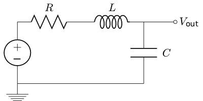
The transfer function H(s) is

\[ H(s)=\frac{\frac{1}{sC}}{R+Ls+\frac{1}{sC}} = \frac{1}{s^2 LC + sRC +1} \]

H(s) already contains the magnitude and phase information of the filter response because

\[ s = \mathrm{j} \omega \]

Second-order filters

The number of poles of the transfer function (the number of roots in the denominator of the transfer function) above determines the order of the circuit. So for the simple LCR circuit above, it is second order. For high-order filters the design principles are very similar.

The transfer function of the second order second-order filters can be written as (Equation B)

\[ H(s) = \frac{H_0}{b_2 s^2 + b_1 s + b_0} \]

where H0 is the gain. Filters can be implemented with different types of components: they can be made up of passive resistors, inductors and compacitors, they can have active components like op amps, or they can be transmission lines, etc. But in the end the transfer function form as in Equation B is the same. The details of implementations set the values of coefficients b2, b1 and b0.

Butterworth, Chebyshev and Bessel filters

Ideally filter should have flat passband, abrupt transition from passband to stopband, and no phase change in the output. However, not surprisingly, real-life filters are not like that. You cannot have all of the desired quality at once; so trade-off has to be made.

Butterworth, Chebyshev and Bessel filters are three commonly used different types of filters that take different compromises in the magnitude response and phase response trade-off. Bessel filter has flat phase response in passband, but slow transition from passband to stopband in magnitude response. Chebyshev filter is just the opposite: fast roll-off from passband to stopband at the cost of some oscillation in passband (or stopband depending on Chebyshev filter type) in magnitude, and uneven phase response. Butterworth is something in the middle, which has flat passband response in magnitude with slower roll-off than Chebyshev filter, and not as flat phase response as Bessel filter.

There are a whole set of mathematical theories behind these filters. And they can be implemented differently. But as being said above, these three types of filters are just different in the way of choosing coefficients of transfer function as in Equation A, and Equation B if they are second-order.

For one benefit of talking about filters in s-domain is that we can write Equation B in a different form (Equation C):

\[ H(s) = \frac{H_0}{(\frac{s}{\omega_0})^2 + \frac{1}{Q} \frac{s}{\omega_0} + 1} \]

where \( \omega_0 \) is the cut-off frequency, and Q is the quality factor of the circuit.

Q factor is an important parameter. Different Q factors are related to different circuit response. An intuitive plot is (taken from Ref 1)

Q factor plot

For example, Butterworth filter has a maximum flat passband response. The corresponding Q factor is \( \frac{\sqrt{2}}{2} \).

Filter prototyping

If the transfer function form of a low-pass filter is known, the “corresponding” transfer functions of high-pass, band-pass and band-stop filters can be easily derived. Take the low-pass filter specified by Equation C for example:

To high-pass filters,

\[ \frac{s}{\omega_0} \rightarrow \frac{\omega_0}{s} \]

To band-pass filters,

\[ \frac{s}{\omega_0} \rightarrow Q (\frac{s}{\omega_0} + \frac{\omega_0}{s}) \]

where \( \omega_0 \) is the passband center frequency.

To band-stop fitlers,

\[ \frac{\omega_0}{s} \rightarrow Q (\frac{s}{\omega_0} + \frac{\omega_0}{s}) \]

where \( \omega_0 \) is the stopband center frequency.

Sallen-Key implementation

Sallen-Key structure is a type of active circuit topology to realize a second-order system with only one op amp. It is widely used. Sallen-Key structure can be easily cascaded to produce higher order system.

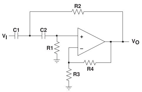
The general Sallen-Key structure is as follows (taken from Ref 2):

general Sallen-Key topology

Ususally Z1, Z2, Z3 and Z4 are either resistors or capacitors, and different combinations give different filter types. Resistors R3 and R4 are responsible for the gain.

The Sallen-Key implementation of low-pass fitlers is like this (Ref 2):

Sallen-Key low-pass

Its transfer function is (Equation D1):

\[ H(s) = \frac{H_0 \frac{1}{R_1 R2 C_1 C_2}}{s^2 + \frac{R_1 C_1 + R_2 C_1 + R_1 C_2 (1-H_0)}{R_1 R2 C_1 C_2} s + \frac{1}{R_1 R2 C_1 C_2}} \]

The Equation D1 above can written in form of cut-off frequency and Q factor as this (Equation D2):

\[ H(s) = \frac{H_0 \omega_0^2}{s^2 + \frac{\omega_0}{Q} s + \omega_0^2 } \]

where

\[ \omega_0 =\frac{1}{\sqrt{R_1 R2 C_1 C_2}} \]

and

\[ Q = \frac{\sqrt{R_1 R_2 C_1 C_2}}{R_2 (C_1 + C_2) + R_1 C_2 (1-H_0)} \]

Equation D2 is very useful since it relates the transfer function with Q and \( \omega_0 \). It also made it easy to work with the filter design table in Ref 3.

The Sallen-Key implementation of high-pass fitlers realized by swapping R1 and C1, R2 and C2 in the low-pass counterpart, as follows (Ref 2):

Sallen-Key high-pass

with transfer function

\[ H(s) = \frac{H_0 s^2}{s^2 + \frac{\omega_0}{Q} s + \omega_0^2 } \]

The formulas for Q and \( \omega_0 \) are the same to the low-pass filter.

Reference

Ref 1: Basic Linear Design, Chaper 8 Analog Filters, from Analog Devices
Ref 2: Analysis of Salley-Key Architecture (Rev.B), from Texas Instruments
Ref 3: Filter design table as a part of Ref 2